Color based detail map blending 1

This method use base color map and selected sample colors to blend the detail maps to the

target area.

This methods allow auto blending any numbers of  detail maps into one base map. The process

does not need interfere from artists but also can be interfere by artist if necessary.

Steps

Step 1 : color extracting

Decide how many detail map you want to use in the final blend and extract color from the base

abedo.

We run color quantization tool to extract selected numbers of colors mostly used in the image.

This example is using 2.

To visualize the color:

Step 2 : choose detail map and feed data to the shader.

Keep in mind that the color is the area where the corresponding maps will be filled in. In this

example brown is where earth texture will be blended in, green is where the grass will be

blended in.

Assign the color and corresponding detail maps to the shader.

Step 3: adjust blending methods according to need.

Blend Strength ：base abedo and detail map blending weight

from 0 to 1

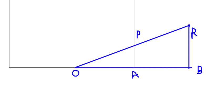
Blending power ：how sharp the blending edge is

from 9 to 29

D1 / D2 value : blending area control

D1 :  from to

Further thinking

Compare to blend map

Color based blending:

  1. Production process is easier and faster , no need to create blend map.

2. Less memory footprint,  no need to store extra map.

3. In theory can blend in any numbers of detail maps.

4. Real time blend area control.
5. Different base map with similar color can use same setting without recalculate.

Blending map :

   1 . Have more control over how to blend.

2 . Requires less calculation on shader.

3.  Can overlay several detail map easily.

Vertex painting

This technique can used together with either Color based blending or blend map to give large

area of control.

Color extraction

Color quantization algorithm extract mostly used colors in a map. While most pixels are covered

in the palate, it has some problem.  

1 . feature colors could be ignored.

This is a test made with extracting 3 main color. The blue dot is too small (too few pixels) to be

count into the main colors.

2. Inaccurate gradiency.  To give a correct gradient on the detail map blending, it’s best to use extreme colors. However due to the character of the algorithm, more average colors are use.

These are the directions to improve the quantization algorithm.

HLSL tutorial : Add reflection

real-time reflection

In real world,  a reflection of and object comes from the environment around it. Offline rendering uses ray trace technique to calculate accurate what's around the target object. In real time rendering shader can use cube map to mimic environment around it and accelerate the calculation of reflection.

I am talking about the implementation of cube map in this chapter.

cube map

A cube map is made from 6 square image. 

When used, you can understand it as : each square image is apply to oneside of the virtual skybox that is surrounding the target object. Althoughthe sky box does not actually exist, but think it in this way help you to understand how the sampling and reflection works.

sampling 

In HLSL, cube map is like any other kinds of texture that can be sampled and used in a shader. Instead of using UV coordinate, cube map use direction to sample.  

 understand it in this way : to sample a cube map, we set a point at the center point of the skybox, then, we start a line at direction R, when the line hit the cube map, the color on the texture on the skybox is the result.

reflection

To correctly sample the cube map to create the reflection effect. We need the reflection vector of the view vector as shown in the following image. The angle between the view vector and normal and the angle between the reflection angle and normal is the same.

the equation to get the reflection :

Reflection = view - 2 x dot (View ,  Normal)  x Normal

or we can simply use reflect ret reflect(i, n) function to calculate. 

implementation

With the basic knowledge above, the implementation is very straight forward:

reflect objects around

Using cube map can reflect a predefined environment but can not reflect the object surround the reflective object.

A way to achieve this is using reflection prob.

A reflection prob defines a point in the environment that render the surrounding environment into a cubemap that can be later used in the shader. The look of the cubemap heavily depends on the view point of the cube map. In real world the cubemap need to be rendered per fragment, but it is unrealistic at runtime. This cause a problem : the reflection is not accurate due to the wrong cube map is used.

parallax-correction cubemap

This technique require artist define the edges for the cub map sampling point. and use the distance between the sample point and reflection point to approximate the correct cube sampling vector from the sample point.

a good reference


R: the real reflection vector
R' : the approximate sample vector on sample point C

calculate the R' (CP)
W is the looking at point on the ground , WP is the reflection vector
CP = WP  - WC

WC = C - vertex position

to calculate WP :
we know that it is on the same direction on the reflection vector R but has a unknown length.
we can say:
 WP = R * scaler;


as shown in the image,
OR/OP = OB/OA = OR(x) / MaxBox(x)

scaler =   MaxBox(x) /OR(x) 

HLSL tutorial : Create capsule light

line light

When calculating point light and direction light,  we take the light as a point. and we use the point to calculate how much the object is lighten by the light. For capsule light we treat the light as a Line, every point on the line can lid the scene.

Algorithm

Here's the strategy to calculate the intensity of the light on one pixel.

Given line AB the presentation of the light, 

To calculate light intensity on pixel P, we need to find the closest point O on line AB and treat O as the only point which lid P. 

This means after we find out point O, the lid model is simplify as a point light. (right image)

Math

To implement this Algorithm we need to map position of P (float3) to O (float3) on AB.

Look at it closely, we can find out the point O is always on line AB. Given the fact that we know vector AB,  as O moves along along AB, the scale M = AO / AB is changing from 0 to 1. When O == A, M = 0; when O ==B, M = 1. As long as we can get the scale calculate, the problem is solved.

Now the equation should be something look like this:

O = A + M (normalize (AB)) ;

to get the point O on AB, we start from point A and displacement along AB vector with M . 

we know:

M = dot (AP, normalized(AB)) * length(AB);

0 <= M <= length(A, B)

Now , Think about these 2 extreme cases :

 

In case 1 : scale M < 0; A is the closest point

case 2 : scale M > length(A, B); B is the closest point. 

we can do some math to map M's value to [0,length]

M = saturate(dot (AP, normalized(AB)) )* length(AB);

code

HLSL tutorial : Create spot light

This article is about how to implementing spot light in HLSL.

Understanding

Attenuation

Different light type has different light attenuation.  Attenuation is describing how light intensity is falloff relate to angle / position and so on.

Inner corn  &  Outer corn 

A spot light has two major parameters that make it different from other kind of light. Inner corn and outer corn. They are shown as 2 yellow corns in the image. 

Corn Attenuation

light inside the inner is 100% intensity.

light get dimmer as it  get closer to the outer corn. 

light get 0% intensity when out of the outer corn.

Math

mapping the range
when doing mapping, 0 is a very important value. Because 0 scale by any value is zero. This will give you a point on the chart that will not move.

to achieve the corn Attenuation, we need a function that take angle (0~Pi) as input and turn it to attenuation (0~1)

The best way to do it is use cos. This map the input from (0~Pi) to (1~0)

Given the target angle is  : Theta

Now we have : Cos(Theta)

When Theta is larger than Out, we want the result to be 0. We achieve this by moving the curve down by Out.

Now we have : Cos(Theta)-Cos(Out)

The next step is quite obvious, we scale the curve up . The scale factor will be 1/(cos (In) - cos(Out)). Because we want the Cos(In) to be one. Then we can saturate the number to get the range we want. 

calculate Cos(Theta)

As can be seen , given the factor that the Light vector and Light to vertex vector is normalized, cos(Theta) = ab / 1. and ab is the projection of Light to vertex vector on light vector, which is dot(light to vertex , light direction). 

Implimentation

As we know all the math by now,  the implementation is quite straight forward : 

you can check the source code here

A test rendering:

As can be seen the bunny is dimmer when they are further away from the center