PBR theory and implementation 2

The model used for f(s)is Cook-Torrance

Cook-Torrance approximates the amount of reflected light considering two factor : microfacet and fresnel effect. The equation is :



In this equation Wo is the viewing direction, Wi is the incoming light direction D F G are the three factors affect how much light will be reflected.

D : normal distribution function

F : Fresnel equation

G : Geometry function

microfacet theory

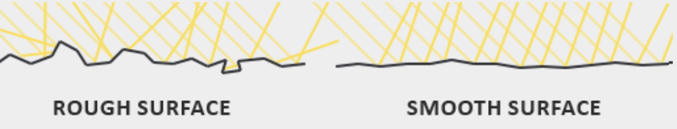
D and G is related to the microfacet theory. The amount of light is reflected relates to smoothness of a surface.

More micro surfaces with reflect vector aligns to the viewing direction more light is reflected to that direction.

More rough the surface , more shadow the surface is casting on itself.

D : Towbridge-Reitx approuch

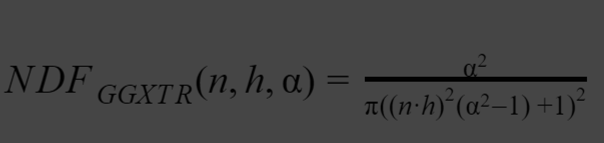
approximate how much microfacets with reflect vectors align to view direction with a given roughness.

𝛂 : roughness * roughness

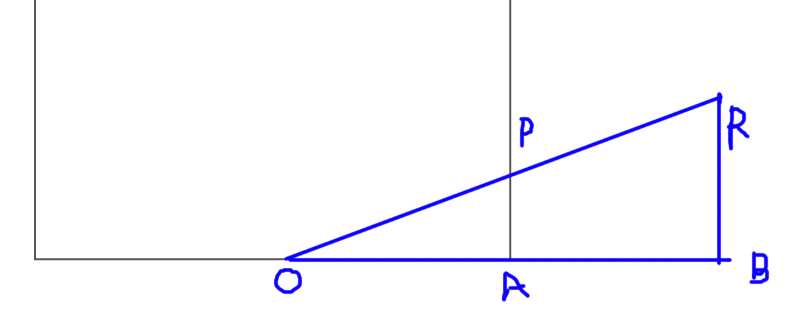
h : normalize (L+V)

n : normal of the surface



h= L+V / length (L,H) = normalize (L+V)

This comes from Blinn_Phong lighting model, instead of evaluating the alignment between view vector and reflect vector, evaluating the Normal vector and Halfway vector of incoming light and view direction.

The correct implimentation of D will be look like :

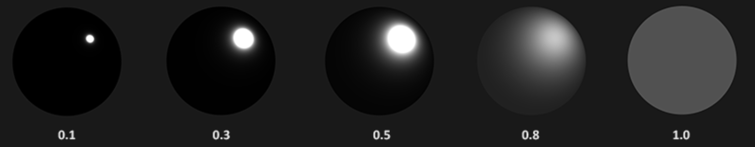
G : Schlick - GGX approximation

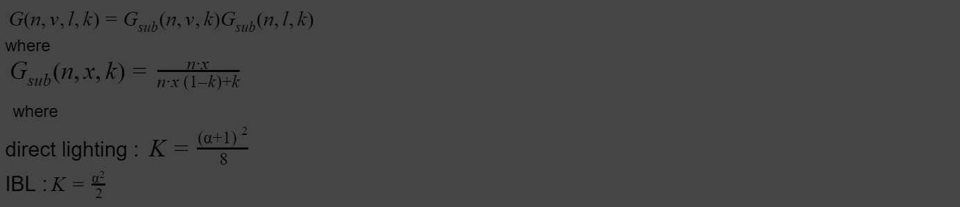
It approximate how much self shadowing will generate given a certain roughness lighting direction and view angle.


The reason it is calculated twice on light vector and view vector is that both of these are affecting how much shadow can be seen.

k is a remapping for . Different lighting situation will need different remapping.

The correct implimentation of G will be look like :

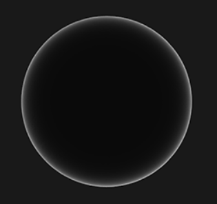
Fresnel schlick approximation

Fresnel equation describe how much light is reflected given a viewing angle and the base reflectivity.

Fresnel effect : the amount of reflected light changes with viewing angle. At grazing angle all material can fully reflect light.


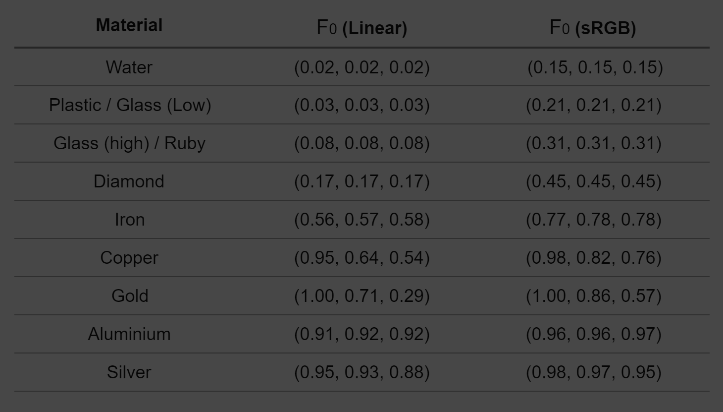
Base reflectivity F0 : describe how much light is reflected when viewing angle is aligned to a surface normal. Different material will have different base reflectivity.

Metal has a higher F0(0.5~1.0) , usually tinted(it is a sRGB). Dielectricity has lower F0(<0.17)

a useful reference chart can be found here





we lerp the value between reflectivity of metall F0-SRGB and a reflectivity of dielecctric 0.04 with the value of the metalic.

The second equation

Distribute outgoing light energy according to the material and form. For example, metal reflect environment much more than dielectric material. It also has a fancy name : BRDF.



correct implimented Fresnel schlick approximation will look like this



When implimenting the equation, we found the precious equation is not matermaticcaly correct , if we use cook-torrance BRDF , because cook-torrance already include the Ks part (how much light is reflected) by having fresnel equation.
Thus , the equation change from :
Lo =(Kd*f(d) +Ks*f(s) ) * Li

to :

Lo =(Kd*f(d) +cook-torrance ) * Li

PBR theory and implementation 1

This article is mainly for my own studying, thus only very key fact will be explain here.

My implementation is in HLSL DirectX 11 in 3ds max environment.

You can see the result in the following image

reference

I read through a lot of article many times to fully understand the theory as well as the math behind this. The ones I reference a lot is :


Very good open gl PBR tutorial

https://learnopengl.com/PBR/Theory

many images in my notes is from here as well

Unity shader source code

Since I want to concentrate on shading I didn’t implement precalculate radiance map and lut this time, I reference Unity’s implementation on real time IBL.

what is PBR ?

Normally you see result images like this when talking about PBR



PBR stands for Physically Based Rendering : The way we calculate the lighting and shading (how different material react to the lighting) follow the physical rules. This will divided the topic into two parts : PBL (physically based lighting ) and PBS (physically based shading)

The target of rendering is : Calculate the light on a surface point by knowing the surface point(p), incoming light direction(i) and strength(Li), view direction(o).

Lo(p,o ) = f(p,i,Li,o)




Traditional lighting model and PBR is doing the same thing but PBR calculate more factors to simulate the real life result.

Energy conservation

One key rule : The radiance(light) comes out from one object can never exceed the light hit on the object.


outgoing light = incoming light

specular and Diffuse distribution

outgoing light from a lit surface falls into two parts : specularand diffuse.





yellow : specular, Light directly get reflected.

red : diffuse , Light get absorbed then comes out from the surface again.


different speculator/diffuse distributions defines the look of different material.


Metal only has speculator, because all the light energy that goes into the surface get absorbed.


To render physically correct means to find the correct distribution between diffuse and specular. In math term it will be something like this:


outgoing light =(diffuse scale+ specular scale) incoming light


because of Energy conservation.


diffuse scale+ speculator scale =1

Material and angle distribution

The next step will be calculate the outcoming light value (r,g,b) given a vertain viewing angle (w0) , incoming light direction (wi) , surface condition (roughness) and material (gold , mud ..)

In other words, how the roughness, metalness, viewing angle , normal ... affect the final result of the outcoming light. How is gold different from mud.

I call it disreibution for now,

view angle light =(diffuse fraction* diffuse distribution + specular fraction* specular distribution) * incoming light

let’s put :

Kd : diffuse fraction

Ks : specular fraction

Li: incoming lighti

Lo : out going light at o

f(d):diffuse distribution

f(s):specular distribution


the equation will be like:


Lo =(Kd*f(d) +Ks*f(s) ) * Li


The reason we seperate f(d) and f(s)is diffuse distribution is different from specular distribution.

In diffuse distribution we use Lambert law (viewing angle does not affect the light value )
In specular , cook-torrance (an advanced relflect / mirror effect)

Render equation

Lo =(Kd*f(d) +Ks*f(s) ) * Li is the Render equation

and Kd*f(d) +Ks*f(s) is the BRDF

BRDF

BRDF Bidirectional reflective distribution function approximates how much each individual light ray i contributes to the final reflected light of an opaque surface given its material properties.


the one used in real time rendering is Cook - Torrance BRDF.


The model used for f(d)is Lambert diffuse : The apparent brightness of a Lambertian surface to an observer is the same regardless of the observer’s angle of view.


f(d) = C/Pi


C is the albedo.

Color based detail map blending 1

This method use base color map and selected sample colors to blend the detail maps to the

target area.

This methods allow auto blending any numbers of  detail maps into one base map. The process

does not need interfere from artists but also can be interfere by artist if necessary.

Steps

Step 1 : color extracting

Decide how many detail map you want to use in the final blend and extract color from the base

abedo.

We run color quantization tool to extract selected numbers of colors mostly used in the image.

This example is using 2.

To visualize the color:

Step 2 : choose detail map and feed data to the shader.

Keep in mind that the color is the area where the corresponding maps will be filled in. In this

example brown is where earth texture will be blended in, green is where the grass will be

blended in.

Assign the color and corresponding detail maps to the shader.

Step 3: adjust blending methods according to need.

Blend Strength ：base abedo and detail map blending weight

from 0 to 1

Blending power ：how sharp the blending edge is

from 9 to 29

D1 / D2 value : blending area control

D1 :  from to

Further thinking

Compare to blend map

Color based blending:

  1. Production process is easier and faster , no need to create blend map.

2. Less memory footprint,  no need to store extra map.

3. In theory can blend in any numbers of detail maps.

4. Real time blend area control.
5. Different base map with similar color can use same setting without recalculate.

Blending map :

   1 . Have more control over how to blend.

2 . Requires less calculation on shader.

3.  Can overlay several detail map easily.

Vertex painting

This technique can used together with either Color based blending or blend map to give large

area of control.

Color extraction

Color quantization algorithm extract mostly used colors in a map. While most pixels are covered

in the palate, it has some problem.  

1 . feature colors could be ignored.

This is a test made with extracting 3 main color. The blue dot is too small (too few pixels) to be

count into the main colors.

2. Inaccurate gradiency.  To give a correct gradient on the detail map blending, it’s best to use extreme colors. However due to the character of the algorithm, more average colors are use.

These are the directions to improve the quantization algorithm.

HLSL tutorial : Add reflection

real-time reflection

In real world,  a reflection of and object comes from the environment around it. Offline rendering uses ray trace technique to calculate accurate what's around the target object. In real time rendering shader can use cube map to mimic environment around it and accelerate the calculation of reflection.

I am talking about the implementation of cube map in this chapter.

cube map

A cube map is made from 6 square image. 

When used, you can understand it as : each square image is apply to oneside of the virtual skybox that is surrounding the target object. Althoughthe sky box does not actually exist, but think it in this way help you to understand how the sampling and reflection works.

sampling 

In HLSL, cube map is like any other kinds of texture that can be sampled and used in a shader. Instead of using UV coordinate, cube map use direction to sample.  

 understand it in this way : to sample a cube map, we set a point at the center point of the skybox, then, we start a line at direction R, when the line hit the cube map, the color on the texture on the skybox is the result.

reflection

To correctly sample the cube map to create the reflection effect. We need the reflection vector of the view vector as shown in the following image. The angle between the view vector and normal and the angle between the reflection angle and normal is the same.

the equation to get the reflection :

Reflection = view - 2 x dot (View ,  Normal)  x Normal

or we can simply use reflect ret reflect(i, n) function to calculate. 

implementation

With the basic knowledge above, the implementation is very straight forward:

reflect objects around

Using cube map can reflect a predefined environment but can not reflect the object surround the reflective object.

A way to achieve this is using reflection prob.

A reflection prob defines a point in the environment that render the surrounding environment into a cubemap that can be later used in the shader. The look of the cubemap heavily depends on the view point of the cube map. In real world the cubemap need to be rendered per fragment, but it is unrealistic at runtime. This cause a problem : the reflection is not accurate due to the wrong cube map is used.

parallax-correction cubemap

This technique require artist define the edges for the cub map sampling point. and use the distance between the sample point and reflection point to approximate the correct cube sampling vector from the sample point.

a good reference


R: the real reflection vector
R' : the approximate sample vector on sample point C

calculate the R' (CP)
W is the looking at point on the ground , WP is the reflection vector
CP = WP  - WC

WC = C - vertex position

to calculate WP :
we know that it is on the same direction on the reflection vector R but has a unknown length.
we can say:
 WP = R * scaler;


as shown in the image,
OR/OP = OB/OA = OR(x) / MaxBox(x)

scaler =   MaxBox(x) /OR(x) 

HLSL tutorial : Create capsule light

line light

When calculating point light and direction light,  we take the light as a point. and we use the point to calculate how much the object is lighten by the light. For capsule light we treat the light as a Line, every point on the line can lid the scene.

Algorithm

Here's the strategy to calculate the intensity of the light on one pixel.

Given line AB the presentation of the light, 

To calculate light intensity on pixel P, we need to find the closest point O on line AB and treat O as the only point which lid P. 

This means after we find out point O, the lid model is simplify as a point light. (right image)

Math

To implement this Algorithm we need to map position of P (float3) to O (float3) on AB.

Look at it closely, we can find out the point O is always on line AB. Given the fact that we know vector AB,  as O moves along along AB, the scale M = AO / AB is changing from 0 to 1. When O == A, M = 0; when O ==B, M = 1. As long as we can get the scale calculate, the problem is solved.

Now the equation should be something look like this:

O = A + M (normalize (AB)) ;

to get the point O on AB, we start from point A and displacement along AB vector with M . 

we know:

M = dot (AP, normalized(AB)) * length(AB);

0 <= M <= length(A, B)

Now , Think about these 2 extreme cases :

 

In case 1 : scale M < 0; A is the closest point

case 2 : scale M > length(A, B); B is the closest point. 

we can do some math to map M's value to [0,length]

M = saturate(dot (AP, normalized(AB)) )* length(AB);

code